Georgia Tech CS 4641 - Machine Learning Group 3 Project
Analyzing Unemployment
Matthew K Attokaren, Matthew Oswald, Saikanam Siam, Sanjit Kumar
Motivation
We are currently experiencing the second major economic recession of our lifetimes due to the COVID-19 pandemic. In the age of information, the advancement of machine learning algorithms has allowed us to gain more knowledge from global economic data than ever before [1]. Integrating data analysis with financial data has made tremendous strides in trading, fraud detection, and market forecasting [2]. These same techniques can be applied on large scale macroeconomic data for countries to find patterns between economic policy and statistics, and unemployment [3].
The unemployment rate is a common metric used to describe a recession; however, a recession affects many more aspects of a country’s economy. Our proposal is to use publicly available datasets to collect yearly attributes such as deficit, tax rates, interest rates, minimum wage, etc. and see if there is any clear correlation with the unemployment rate. Our main goal is to identify which factors or policies contribute to an increase in unemployment for countries.
The problem we are trying to solve is how can unemployment rates be predicted using publicly available data of countries’ yearly economic attributes (such as property rights, government integrity, tax burden, etc.) from the past decade?
Why is it important and why should we care?
Economic recessions can have a major negative impact on countries and their citizens. If we can learn which combination of economic indicators can predict a recession and increased unemployment, then governments and people can use this information to better prepare for a downturn and inform economic policy makers.
Additionally, there is a large amount of data available to the public. Economic forecasting is a vital tool for any country to have, and encouraging scientists and researchers to analyze this data could have profound positive impacts on a global scale.
The Dataset
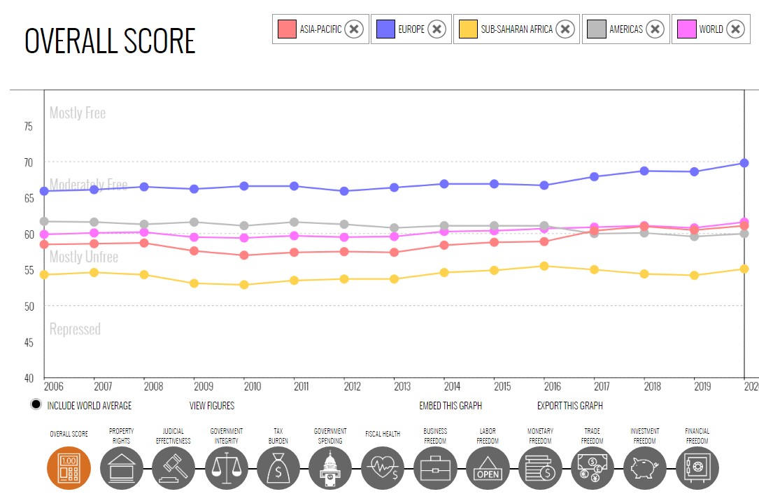
We obtained most of our attribute data set from the Heritage Foundation. The dataset contains thirteen indexes of economic freedom for each year. These indices include Property Rights, Judicial Effectiveness, Government Integrity, Tax Burden, Government Spending, Fiscal Health, Business Freedom, Labor Freedom, Monetary Freedom, Trade Freedom, Investment Freedom, and Financial Freedom. The Heritage Foundation records these indexes from over 150 countries, with some indexes dating back to 1995 for some of the countries.
We then obtained the unemployment rates for each country from The World Bank. This dataset contains the unemployment rates for each country, which we used as our labels. For our linear regression analysis, we also obtained spending, taxes, occupational data (agriculture, industry, services) and interest rates from the world bank.
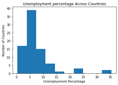
We gathered data on multiple facets of economics that cover economics at a macro level and micro level instead of looking at them individually. Having so many different features reduces the risk of confounding variables skewing our dataset and us not being able to identify them, although this causes one of the primary problems with high-dimensionality also known as model overfitting. This is where PCA comes in. We used PCA to reduce our dataset to two principal components that would maximize the variance between countries. This also allowed us to better visualize our dataset and see if there are any trends:
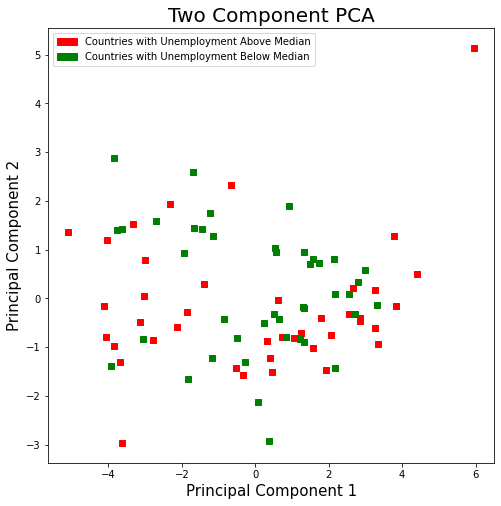
The median unemployment rate for all countries was 5.83%. Using this value, countries were split into two group: countries with unemployment above the median rate and countries with unemployment below median rate. At first glance, there did not appear to be a simple way to seperate countries with high employment from countries with low employment using the two principal components. For future analysis, we would like to use SVM to see if we can create a linear classifier in a higher dimensional space.
We did PCA analysis on the group of freedom attributes. We then created a heat map of the variables that were most influential using PCA:
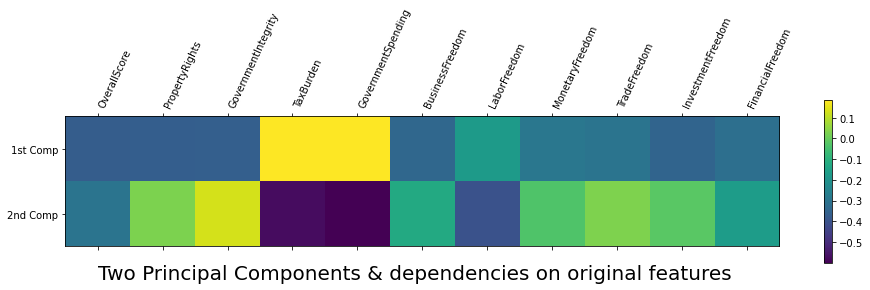
Each principal component is a linear combination of our original features. The figure above illustrates how much each component contributed to the first two principal components. The first principal component accounts for the most variance amonst the countries. The top contributing features for the first principal component were Government Spending and Tax Burden. This means that increased spending from the government along with a higher tax burden both increase unemployment. These findings were similar to our basic linear regression results that we show later and go against Keynesian economics.
Method
First we look at a specific economic policy that was historically suggested and used during the first great depression, known as Keynesian policies. According to Keynesian Economics, there are three main ways a government can stabilize an economy during a recession. One way is to decrease interest rates. This allows easier borrowing for businesses and therefore creates more jobs. The second way a government can increase jobs is by decreasing taxes. This is based on the same idea that additional money in the hands of citizens will allow for more businesses to stay open. The third main way a government can stabilize a recession is by increasing spending to again put more money in the hands of citizens.
In order to analyze these policies, we used Regression and PCA to analyze the impact of Keynesian policies on unemployment. Furthermore, we tried and succeeded to back up some of our claims by finding the most important attribute predictors to unemployment by using PCA. The strong correlations between certain attributes and unemployment indicated to us that we could be able to generate an accurate predictor for unemployment. To evaluate our data, grouped our data into two training sets. We wanted to see if we could use a countries previous years’ data to predict a future year’s unemployment rate. We also wanted to see if we could predict one countries unemployment rate by using other countries’ data.
Our approach to analyzing the countries and yearly data was to break up the time series data into manageable data sets. Our entire data set consisted of 10 years of data, from 2009-2018, each year consisting of 135 countries. Each country had most of the attributes that we used from the Heritage Foundation data, and we used the unemployment statistics from WorldBank.org, specifically the modeled ILO estimate data in order to not have any data gaps. Unlike before, we decided to not include the previous year’s unemployment rate as a feature for the current year’s attributes. We wanted to really see how accurate of a model we could get with just the Heritage data.
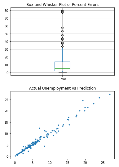
We broke up the time series data by separating by country, then separating by year. We first created a separate DataFrame for every country, each consisting of that country’s data over the 10-year period. Our goal was to see how accurately we could predict the unemployment for a country given the first 9 years. Our testing data was the first 9 years for that country, and our model ran only for the 10th year, which we compared to the actual result. We did this for every country and analyzed the percent error for each country and the sum of squared differences overall. We then created a boxplot and scatterplot for the percent error. We tried many different regression algorithms to see which one would work the best. Normal Linear Regression gave the worst results, with a high sum of squared differences and high mean percent error. We assumed that this would happen, given the complexity of our data, and then tried Kernel Ridge Regression due to the multicollinearity of our data. Additionally, we thought the Kernel Trick would help find more intricate clusters in the data. This was a significant improvement, and our sum of squared differences decimated while the mean percent error was halved. We decided to try more regression algorithms and tune slightly to see the best we can get. We decided to try least-angle regression, which is useful for high-dimensional data. This is good for us, since we had the same number of features as our data, since every country has a separate model. This also helped increase our accuracy. Lastly, we also implemented a Multi-Layer Perceptron Neural Network. Although it required the most tuning, we were able to achieve the best results using the neural network.
Once we knew that Neural Networks worked best for our data, we decided to move on to the next phase of analysis, which is analyzing all the countries on a year by year basis. We decided to hand pick 24 countries that had major affects due to the economic recession of 2008 or had a good trading relationship with the US at the time. The countries we researched and chose are China, Canada, Japan, Germany, United Kingdom, France, India, South Africa, Italy, Israel, Vietnam, Latvia, Chile, Netherlands, Bhutan, Qatar, Turkey, Ukraine, Greece, Belgium, Ethiopia, Lesotho, Zimbabwe, Ghana. We felt like this was a diverse mix of countries and a good subset to test on. We used all the other countries as our training data and ran the algorithm for every year. All of these tests definitely gave us more clarity on what we are able to do and not able to do with the data in hand.
Results
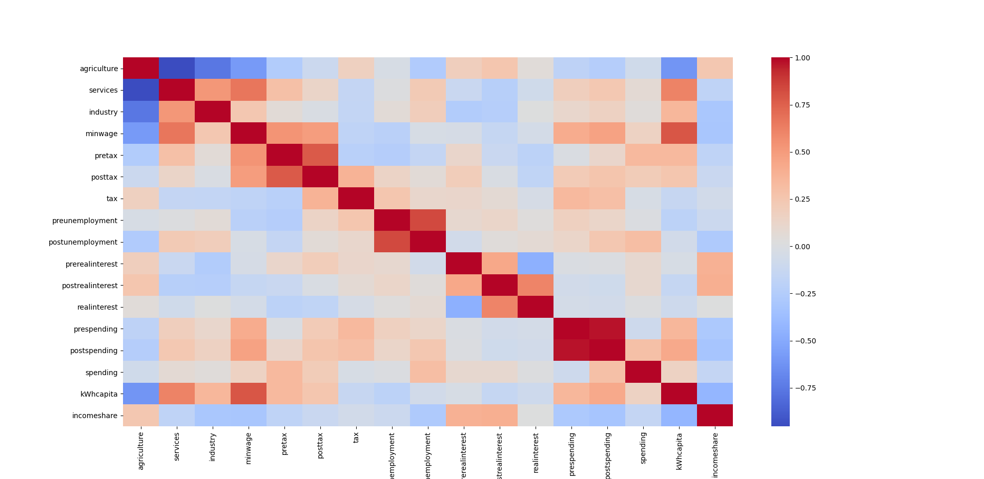
We can notice a couple of basic correlations on the preliminary heatmap. For example, we can see that obviously the more farming an economy has, the fewer service employees the country has. Then we will start to notice other things like the higher the minimum wage, the more energy costs. We can see that the interest, taxes, and unemployment before the recession are correlated to those variables during the recession. The correlations to unemployment are:
Creating a Model to decide Changes One major issue that our team had was that there is a very limited amount of consistent data for the countries. Of the features that we had, the maximum number of data points was 162 and the minimum was 80. This created a necessity to make our model as simple as possible as including all potential features would limit our data to only 23 data points. To ensure we only kept only the most important variables, we created a function much like regsubsets where it chooses the highest R^2 score from possible subsets and we are able to force certain features to be included in R except it accounted for potential blank data points for each combination as opposed to the whole dataset (Our function only seemed efficient enough to work on up to around 200 combinations).
Variables that don’t affect future unemployment: Initial Government Spending (prespending), Change in Real Interest Rates (realinterest), Real Interest Rates (prerealinterest), and Change in Taxation Rates (tax). All of these had P>|t| of .4 or more. Our final model for identifying changes in policy looked like this:
Based on this model, we can choose two policies between monetary and fiscal policy.
Decrease Spending During a Recession: We see that there is no impact on unemployment based on initial spending, but we see that there is a positive correlation between the act of increasing spending and unemployment. This seems like it goes against Keynesian economics, but a possible explanation would be that increased spending makes people wary of the possibility of a country going bankrupt and therefore less advantageous for business. Oftentimes taxes for businesses go up to accomodate the increase in govt. spending, this in turn makes economoic recovery harder.
Increase Taxes on Income, Profits, and Capital Gains Before the Next Recession: We can see that the 2007 tax variable is -.0757X+.0009X^2 If we solve for the minimum, we can see that we can decrease unemployment by up to 1.6% by putting the taxes to 42%.
We then moved on to our prediction algorithms. Our results for each algorithm are as follows. Our final algorithm was able to achieve a mean percent error of around 11.4 percent. We considered this to be a good model, and we think that it is an accurate predictor of a country’s unemployment rate.
| Algorithm | Sum of Squared Differences | Mean Percent Error |
|---|---|---|
| Linear Regression | 2240.569837566454 | 47.89802773067209 |
| Kernel Ridge | 275.0206382935021 | 19.756660299281467 |
| LARS Lasso | 158.78309100163676 | 16.29075920173418 |
| MLP Neural Network | 148.5540210937815 | 11.412074346825115 |
Percent Error for Each Country for Each Algorithm
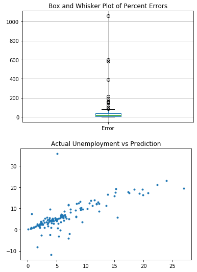
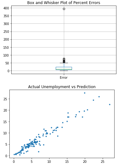
The first chart is a box and whiskers plot for the Percent Error for the countries. It makes it easy to see the minimum, mean, maximum, quartiles and outliers for the data. The number of outliers also decreased as we used better algorithms.
The second chart is a scatterplot that contains the Actual Unemployment rate on the X axis and the Prediction on the Y axis for each country. It is clear to see that as we used better algorithms, the trend line become more concentrated towards the line y=x. This further indicates the increase in model accuracy.
Linear Regression
Kernel Ridge
LARS Lasso
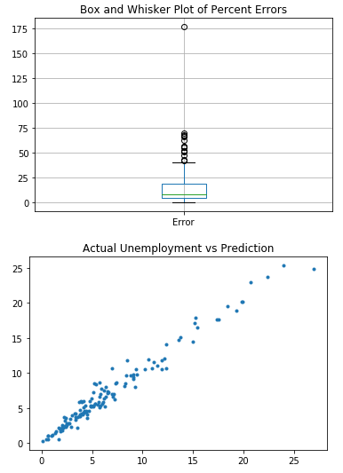
MLP Neural Network
We then analyzed the yearly data and tried to predict the 24 countries’ unemployment using the rest of the countries. Note that this is a different way of analyzing the same data, since we’re analyzing all countries in a year rather than a country over time. We tuned the Neural Network again to obtain the best results we could get, but we did not obtain the high results that we wanted. We scored all the test data for each year using SKLearn and obtained these results.
| Year | Score |
|---|---|
| 2009 | 0.139663 |
| 2010 | 0.242222 |
| 2011 | 0.292534 |
| 2012 | 0.451128 |
| 2013 | 0.308387 |
| 2014 | 0.445866 |
| 2015 | 0.406520 |
| 2016 | 0.252423 |
| 2017 | 0.321830 |
| 2018 | 0.341526 |
After running these tests, we concluded with fair certainty that we were not able to accurately predict a country’s unemployment rate given the year and other countries’ data. This makes sense, since it does not factor in that specific country’s economic confounding variables. The only upside was the four years from 2012-2015 that gave us a fairly accurate result. We do not think that we were able to generate a very good model for this specific purpose. Additionally, we think that adding the previous year’s unemployment as an attribute for the current year would have increased the score, which is something we can look into for the future.
Conclusion and Presentation
At first glance, our findings about economic recovery goes against some of the standard beliefs held in Keyesian theory. Our analysis specifically goes against increasing government spending and high taxation of businesses during economic recovery. Keynesian theory states that the government should step in when there’s an economic downturn, but once it’s on the recovery phase, it should go back to free market policies such as lowering taxes and decreasing spending. Our findings were not in-depth enough to analyze the validity of all of these theories. However, we were able to corroborate from our model that during the recovery phase, increasing government spending is not optimal for long-run economic recovery. A future possibility would be to separate out economic downturn and recovery phase and analyze them individually.
Unemployment forecasting would be an extremely vital tool for countries, and we did our best to create a consistent model that can analyze the Heritage statistics for a country over time to predict unemployment. We are confident by the low mean percent error that our machine learning model was an accurate predictor of a country’s unemployment rate. Additionally, economic downturns in United States affect the rest of the world, and we tried to use this intuition to try to predict the unemployment levels of the global economy year by year during the decade after the economic recession. Our findings definitely fall short when it comes to using one snapshot at a time to look at the global economy and predicting the unemployment of 24 countries just by using the rest of the countries. This makes sense given the huge array of confounding variables and their variabiliy in trade relations between countries, tariffs, sanctions, and types of governments in the entire world. As stated before, we could have improved our results by adding the previous year’s unemployment as a current attribute. This just goes to show how fickle global economic predictions are and why they can often be wrong.
Presentation Link
https://youtu.be/-gZ2_5S99sk
References
-
[1] Athey, S. (2018). The impact of machine learning on economics. In The economics of artificial intelligence: An agenda (pp. 507-547). University of Chicago Press.
-
[2] Puglia, M., & Tucker, A. (2020). Machine Learning, the Treasury Yield Curve and Recession Forecasting.
-
[3] Katris, C. (2020). Prediction of unemployment rates with time series and machine learning techniques. Computational Economics, 55(2), 673-706.
-
[4] Jahan, S., Mahmud, A. S., & Papageorgiou, C. (2014). What is Keynesian economics?. International Monetary Fund, 51(3).